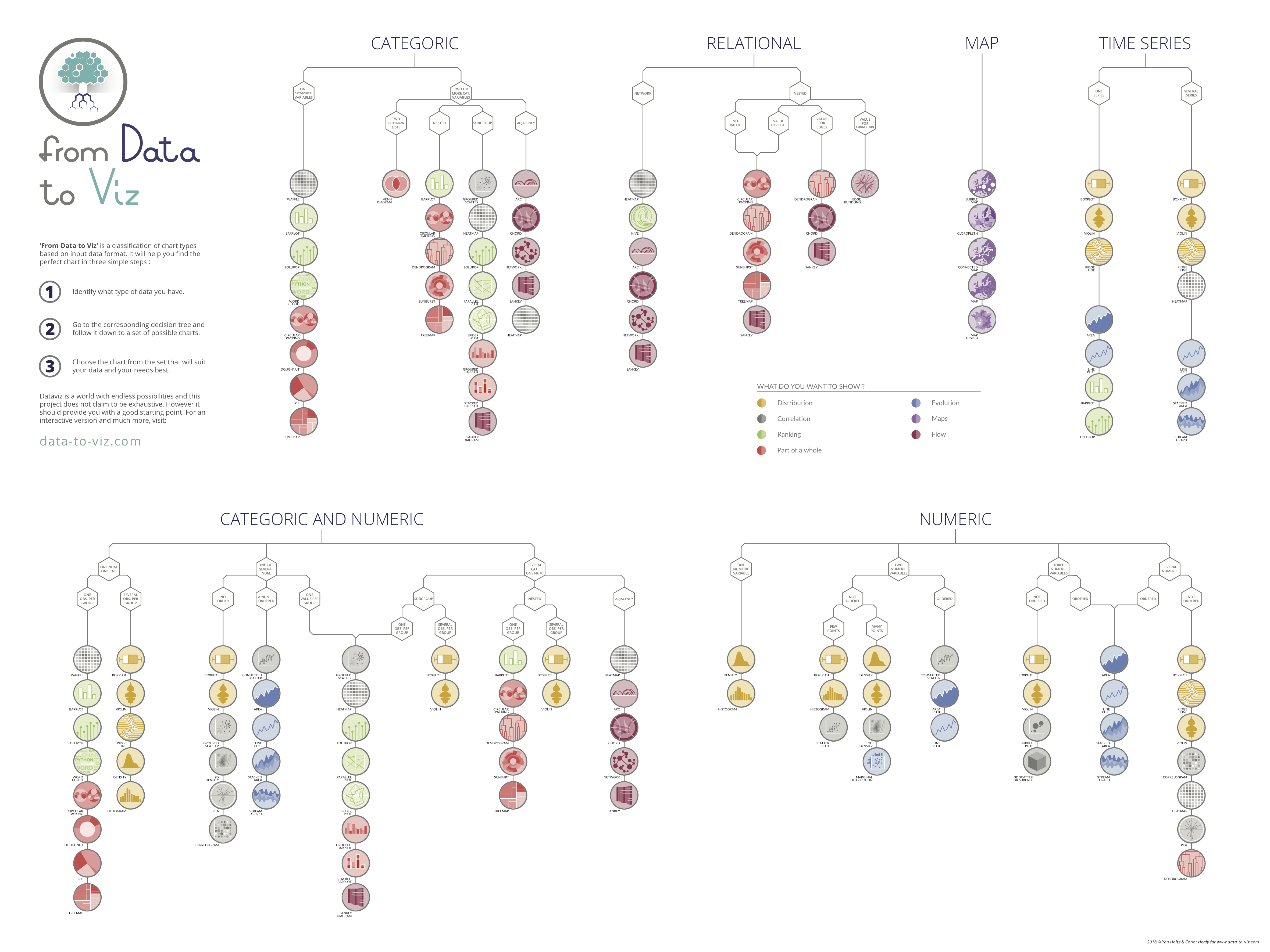
Escolher o tipo de gráfico adequado para os dados é fundamental para garantir uma comunicação clara e eficaz das informações. Cada conjunto de dados possui características específicas, como variáveis contínuas e/ou categóricas, e selecionar o gráfico correto ajuda a destacar padrões, tendências e relações que poderiam passar despercebidos. Um gráfico mal escolhido pode confundir o leitor ou até mesmo transmitir uma interpretação errada dos dados, comprometendo a tomada de decisão baseada neles.
      species          island    bill_length_mm  bill_depth_mm
 Adelie   :146   Biscoe   :163   Min.   :32.10   Min.   :13.10
 Chinstrap: 68   Dream    :123   1st Qu.:39.50   1st Qu.:15.60
 Gentoo   :119   Torgersen: 47   Median :44.50   Median :17.30
                                 Mean   :43.99   Mean   :17.16
                                 3rd Qu.:48.60   3rd Qu.:18.70
                                 Max.   :59.60   Max.   :21.50
 flipper_length_mm  body_mass_g       sex           year
 Min.   :172       Min.   :2700   female:165   Min.   :2007
 1st Qu.:190       1st Qu.:3550   male  :168   1st Qu.:2007
 Median :197       Median :4050                Median :2008
 Mean   :201       Mean   :4207                Mean   :2008
 3rd Qu.:213       3rd Qu.:4775                3rd Qu.:2009
 Max.   :231       Max.   :6300                Max.   :2009
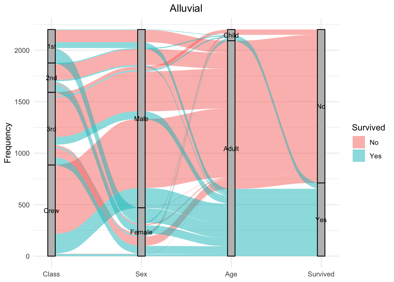
dados2 <-as.data.frame(Titanic)summary(dados2)
  Class       Sex        Age     Survived      Freq
 1st :8   Male  :16   Child:16   No :16   Min.   :  0.00
 2nd :8   Female:16   Adult:16   Yes:16   1st Qu.:  0.75
 3rd :8                                   Median : 13.50
 Crew:8                                   Mean   : 68.78
                                          3rd Qu.: 77.00
                                          Max.   :670.00
dados3 <- gapminder::gapmindersummary(dados3)
        country        continent        year         lifeExp
 Afghanistan:  12   Africa  :624   Min.   :1952   Min.   :23.60
 Albania    :  12   Americas:300   1st Qu.:1966   1st Qu.:48.20
 Algeria    :  12   Asia    :396   Median :1980   Median :60.71
 Angola     :  12   Europe  :360   Mean   :1980   Mean   :59.47
 Argentina  :  12   Oceania : 24   3rd Qu.:1993   3rd Qu.:70.85
 Australia  :  12                  Max.   :2007   Max.   :82.60
 (Other)    :1632
      pop              gdpPercap
 Min.   :6.001e+04   Min.   :   241.2
 1st Qu.:2.794e+06   1st Qu.:  1202.1
 Median :7.024e+06   Median :  3531.8
 Mean   :2.960e+07   Mean   :  7215.3
 3rd Qu.:1.959e+07   3rd Qu.:  9325.5
 Max.   :1.319e+09   Max.   :113523.1
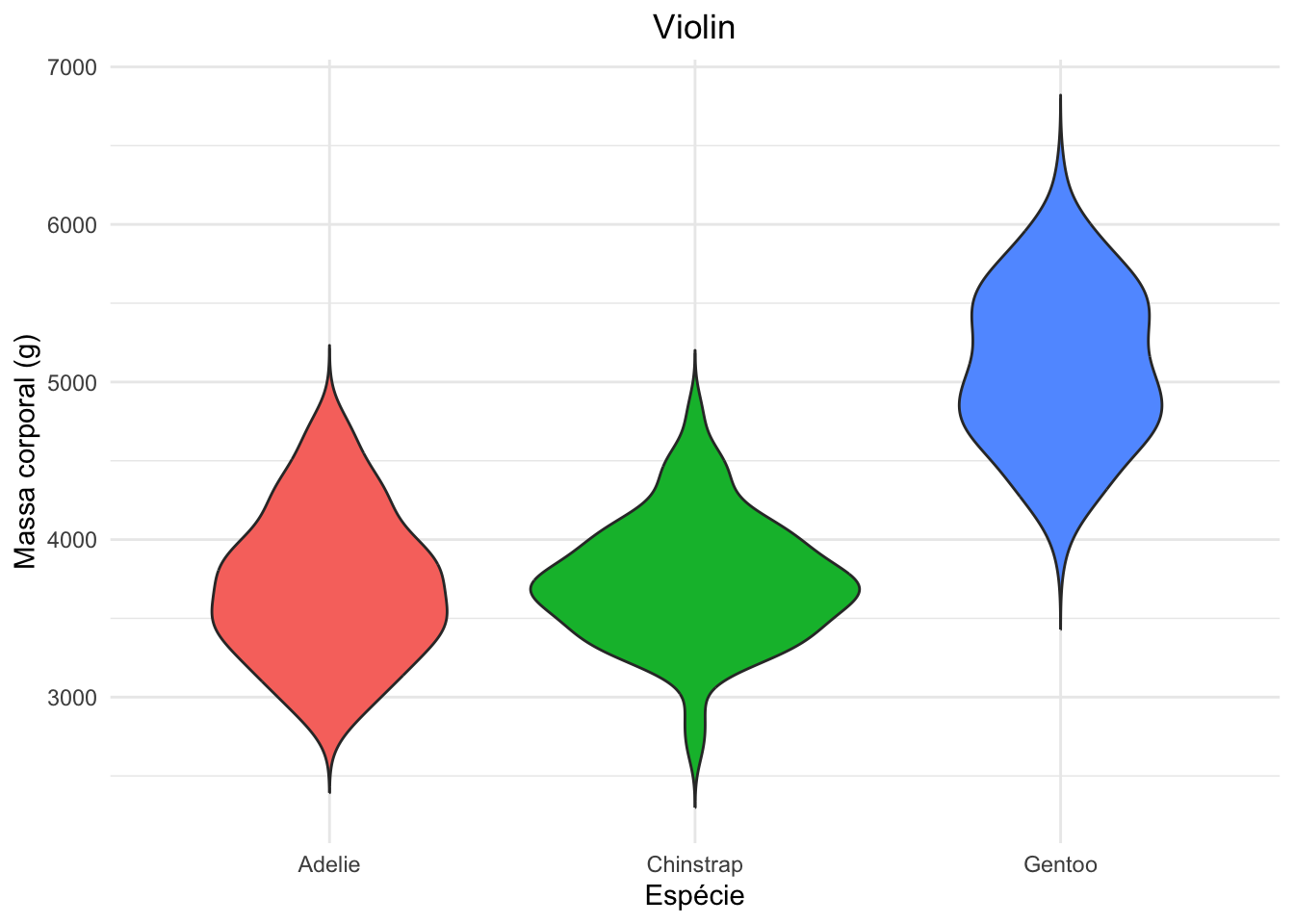
4.1 1 variável numérica
# Violin(g1 <-ggplot(dados1, aes(x = species, y = body_mass_g, fill = species)) +geom_violin(trim =FALSE) +labs(title ="Violin", x ="Espécie", y ="Massa corporal (g)") +theme_minimal() +theme(legend.position ="none", plot.title =element_text(hjust =0.5)))
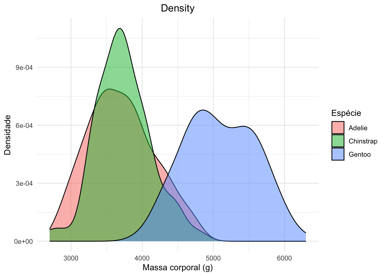
# Density(g2 <-ggplot(dados1, aes(x = body_mass_g, fill = species)) +geom_density(alpha =0.5) +labs(title ="Density",x ="Massa corporal (g)", y ="Densidade", fill ="Espécie") +theme_minimal() +theme(plot.title =element_text(hjust =0.5)))
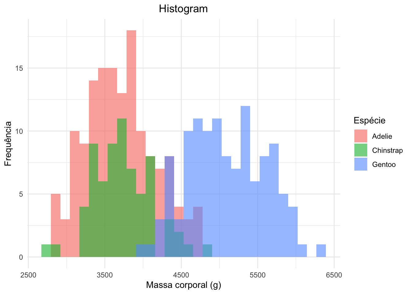
# Histogram(g3 <-ggplot(dados1, aes(x = body_mass_g, fill = species)) +geom_histogram(bins =30, alpha =0.6, position ="identity") +labs(title ="Histogram",x ="Massa corporal (g)", y ="Frequência", fill ="Espécie") +theme_minimal() +theme(plot.title =element_text(hjust =0.5)))
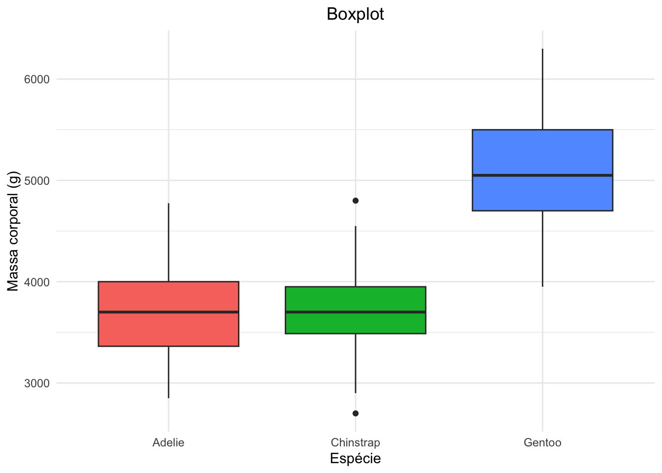
# Boxplot(g4 <-ggplot(dados1, aes(x = species, y = body_mass_g, fill = species)) +geom_boxplot() +labs(title ="Boxplot",x ="Espécie", y ="Massa corporal (g)") +theme_minimal() +theme(legend.position ="none", plot.title =element_text(hjust =0.5)))
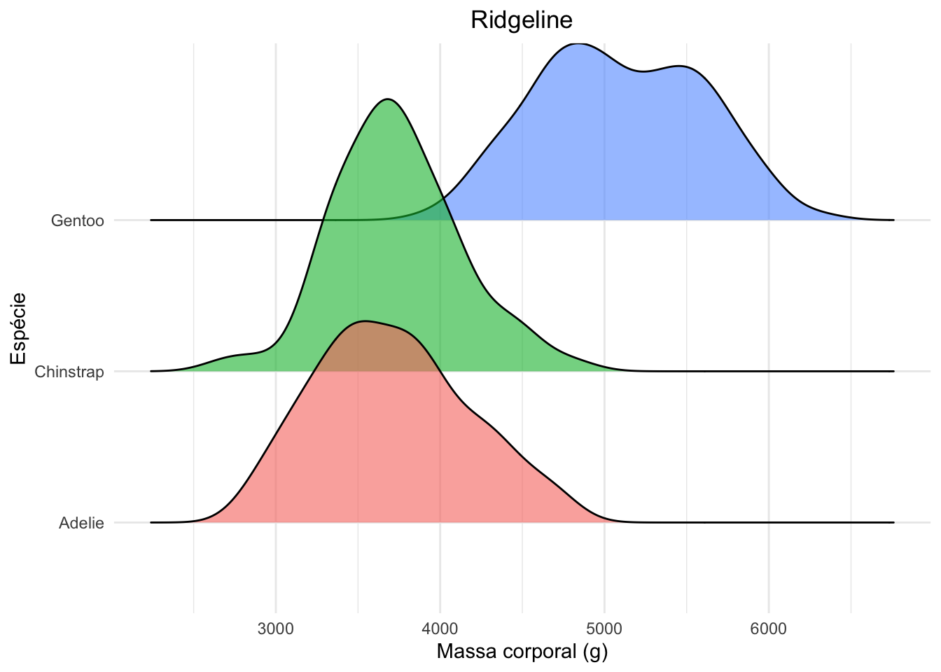
# Ridgelinelibrary(ggridges) (g5 <-ggplot(dados1, aes(x = body_mass_g, y = species, fill = species)) +geom_density_ridges(alpha =0.6) +labs(title ="Ridgeline",x ="Massa corporal (g)", y ="Espécie") +theme_minimal() +theme(legend.position ="none", plot.title =element_text(hjust =0.5)))
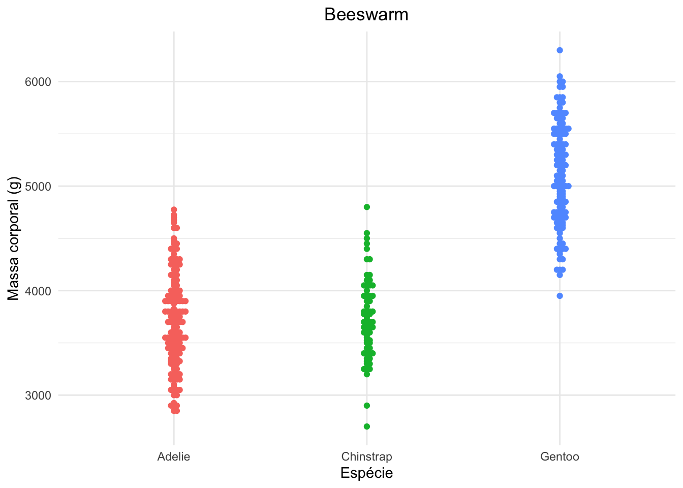
# Beeswarmlibrary(ggbeeswarm) (g6 <-ggplot(dados1, aes(x = species, y = body_mass_g, color = species)) +geom_beeswarm(cex =0.5) +labs(title ="Beeswarm",x ="Espécie", y ="Massa corporal (g)") +theme_minimal() +theme(legend.position ="none", plot.title =element_text(hjust =0.5)))
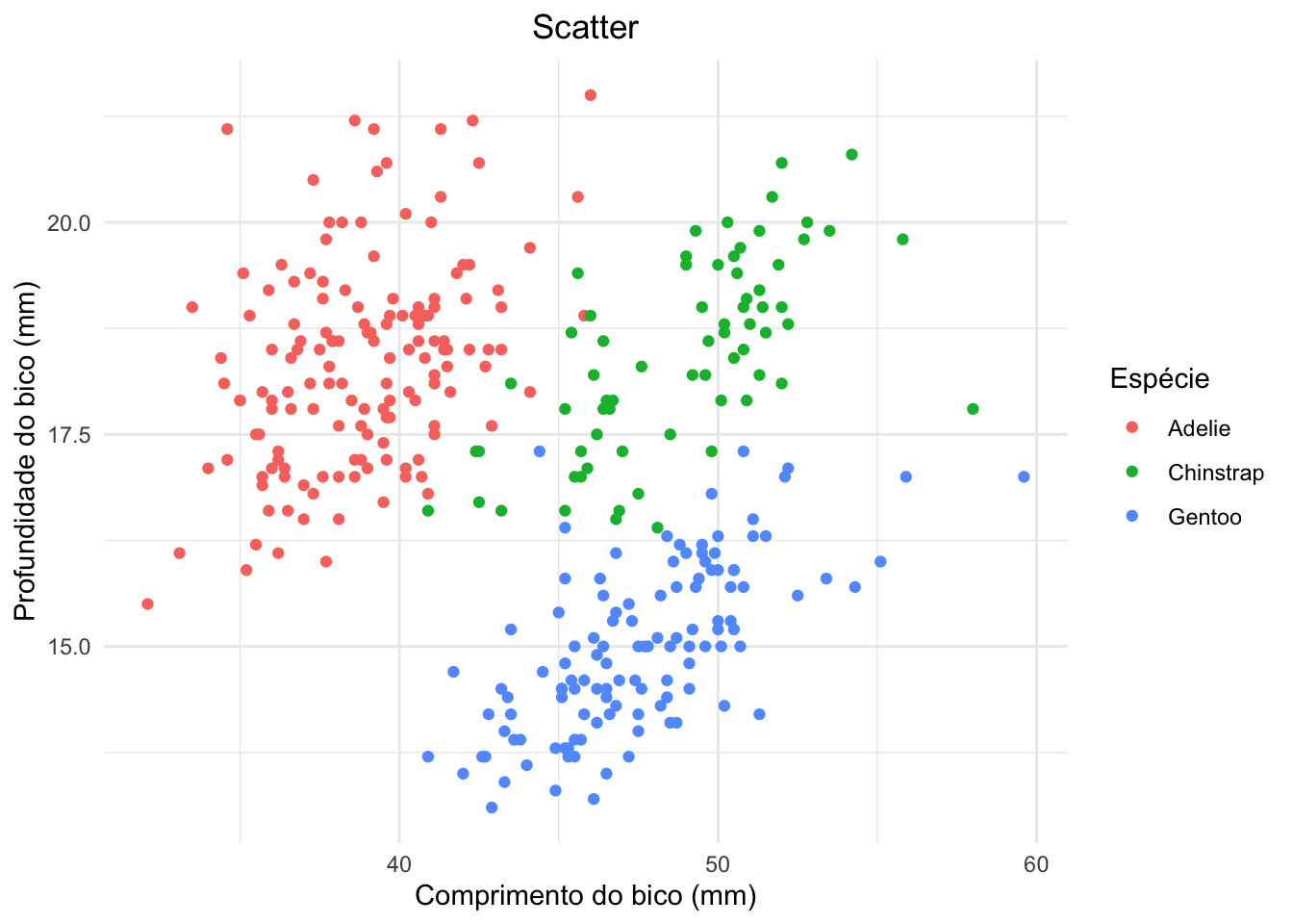
4.2 2 variáveis numéricas
# Scatter(g1 <-ggplot(dados1, aes(x = bill_length_mm, y = bill_depth_mm)) +geom_point(aes(color = species)) +labs(title ="Scatter",x ="Comprimento do bico (mm)", y ="Profundidade do bico (mm)", color ="Espécie") +theme_minimal() +theme(plot.title =element_text(hjust =0.5)))
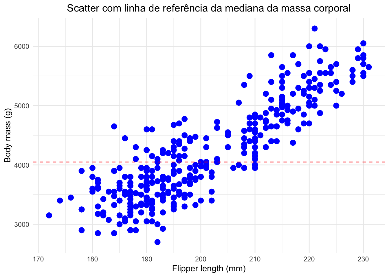
Linhas de referência
(gh <-ggplot(dados1, aes(x = flipper_length_mm, y = body_mass_g)) +geom_point(size =3, color ="blue") +geom_hline(yintercept =median(dados1$body_mass_g),linetype ="dashed", color ="red") +labs(title ="Scatter com linha de referência da mediana da massa corporal",x ="Flipper length (mm)", y ="Body mass (g)") +theme_minimal() +theme(plot.title =element_text(hjust =0.5)))
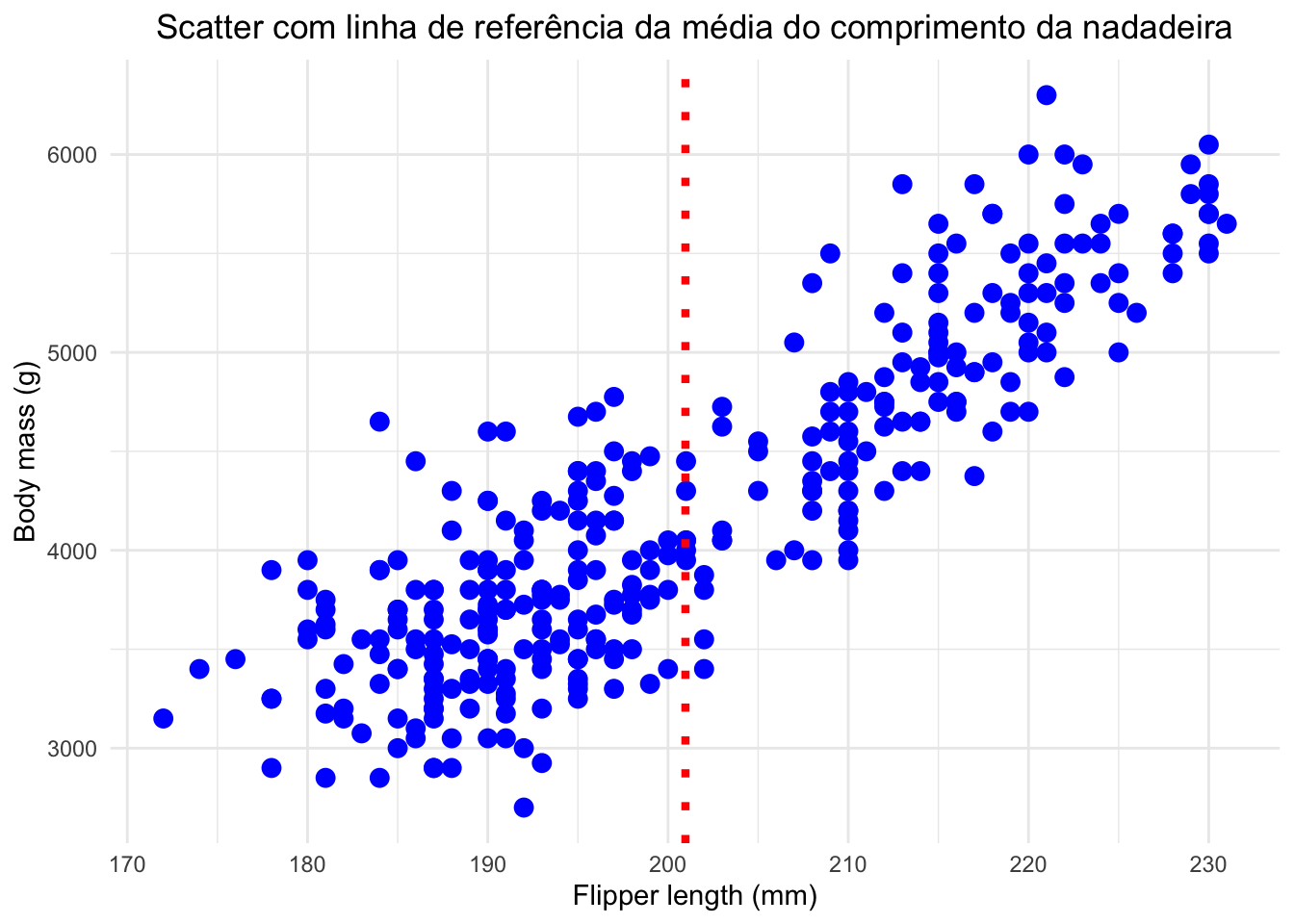
(gv <-ggplot(dados1, aes(x = flipper_length_mm, y = body_mass_g)) +geom_point(size =3, color ="blue") +geom_vline(xintercept =mean(dados1$flipper_length_mm),linetype ="dotted", linewidth =1.5, color ="red") +labs(title ="Scatter com linha de referência da média do comprimento da nadadeira",x ="Flipper length (mm)", y ="Body mass (g)") +theme_minimal() +theme(plot.title =element_text(hjust =0.5)))
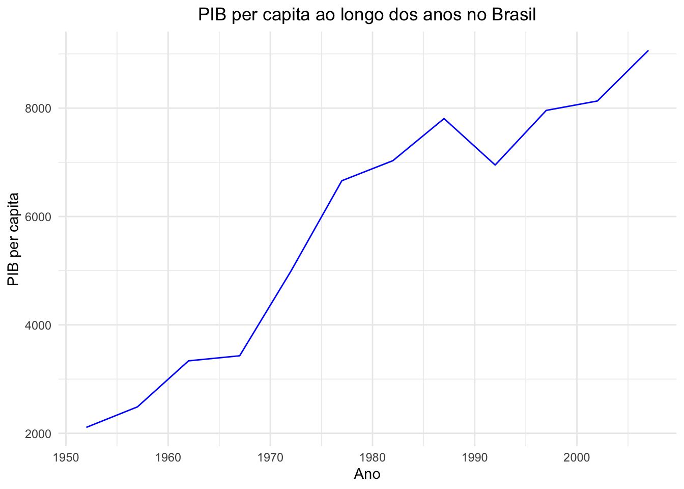
4.3 1 variável numérica e 1 variável categórica
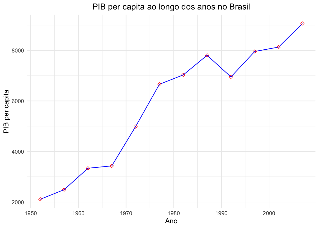
# Line gap1 <- dados3 %>%filter(country =="Brazil")(g1 <-ggplot(gap1, aes(x = year, y = gdpPercap)) +geom_line(color ="blue") +labs(title ="PIB per capita ao longo dos anos no Brasil", x ="Ano", y ="PIB per capita") +theme_minimal() +theme(plot.title =element_text(hjust =0.5)))
g1 +geom_point()
g1 +geom_point(color ="red", shape =5)
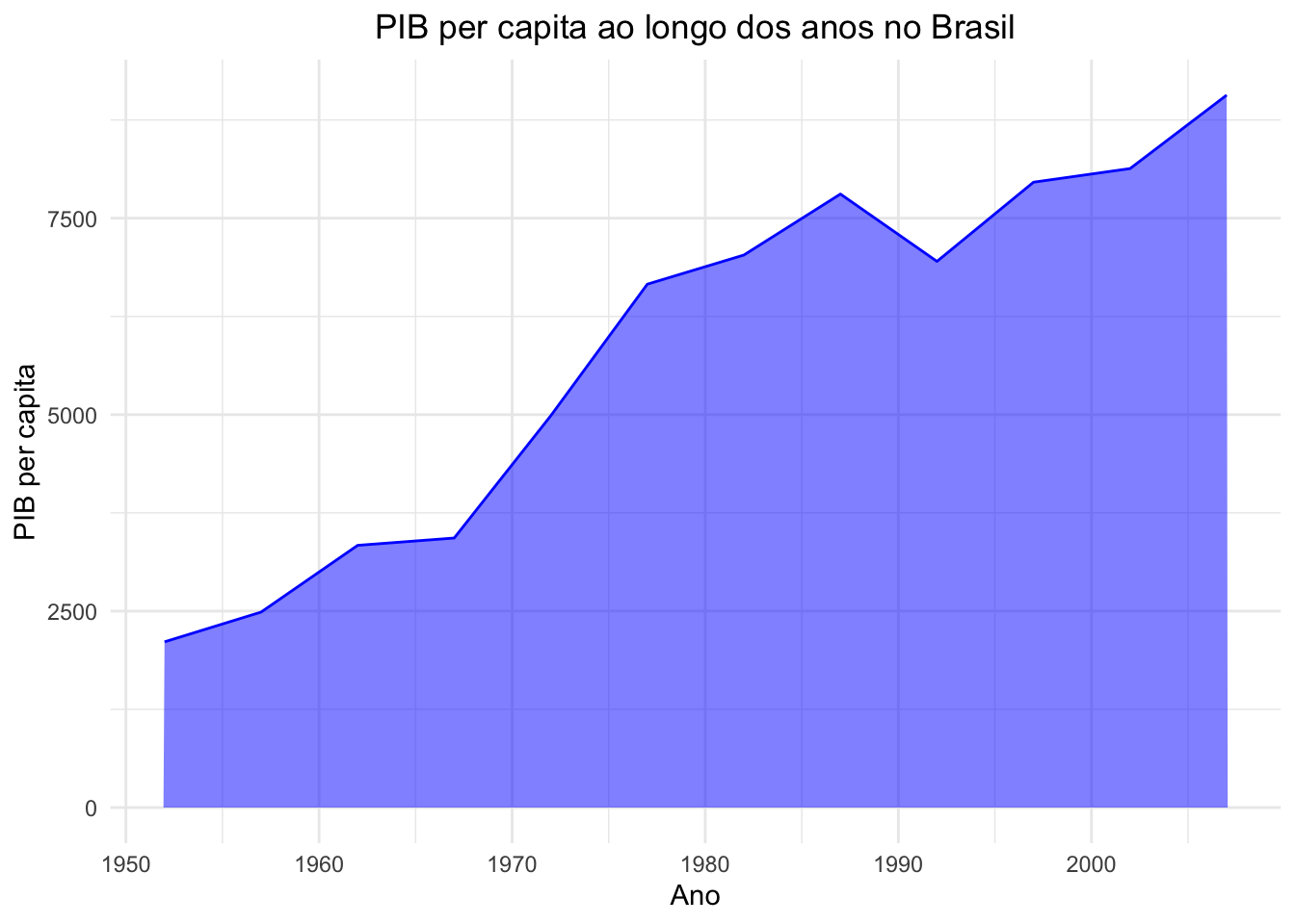
# Area(g2 <-ggplot(gap1, aes(x = year, y = gdpPercap)) +geom_area(fill ="blue", color ="blue", alpha =0.5) +labs(title ="PIB per capita ao longo dos anos no Brasil", x ="Ano", y ="PIB per capita") +theme_minimal() +theme(plot.title =element_text(hjust =0.5)))
4.4 2 variáveis categóricas e 1 numérica
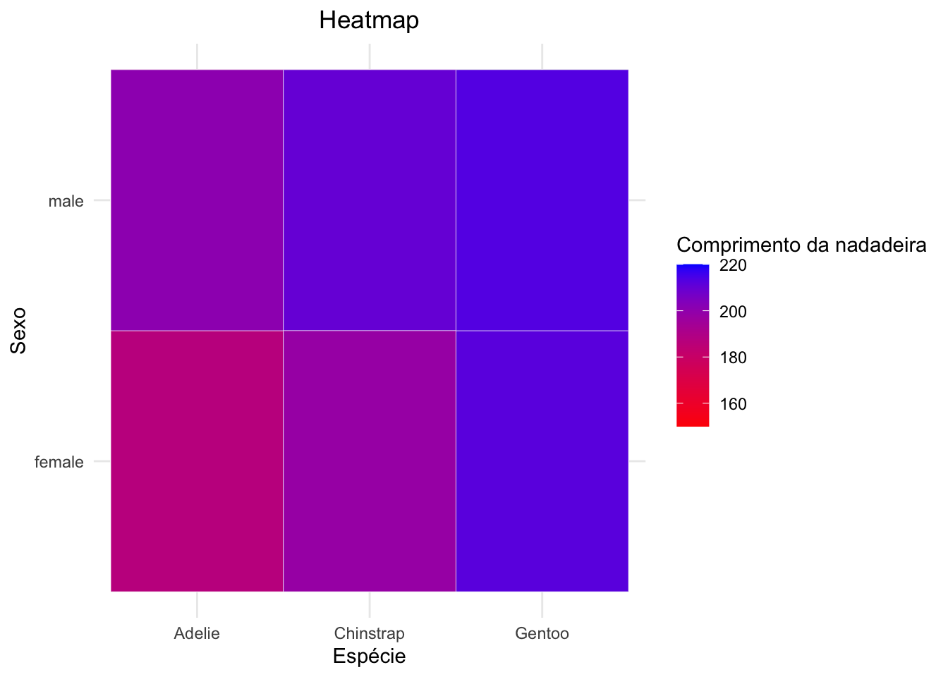
# Heatmapggplot(dados1, aes(x = species, y = sex, fill = flipper_length_mm)) +geom_tile(color ="white") +scale_fill_gradient(low ="red", high ="blue", limits =c(150, 220)) +labs(title ="Heatmap",x ="Espécie",y ="Sexo",fill ="Comprimento da nadadeira" ) +theme_minimal() +theme(plot.title =element_text(hjust =0.5))
# Col - usa os valores que você fornece em yresumo <- dados1 %>%group_by(species) %>%summarise(contagem =n(), .groups ="drop")(g1 <-ggplot(resumo, aes(x = species, y = contagem)) +geom_col(fill ="darkgreen") +labs(title ="Col", x ="Espécie", y ="Contagem") +theme_minimal() +theme(plot.title =element_text(hjust =0.5)))
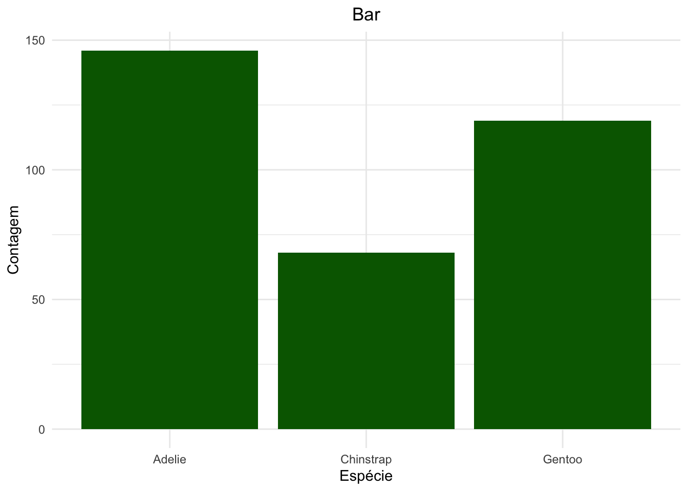
# Bar - calcula contagem automaticamente(g1 <-ggplot(dados1, aes(x = species)) +geom_bar(fill ="darkgreen") +theme_minimal() +labs(title ="Bar", y ="Contagem", x ="Espécie") +theme(plot.title =element_text(hjust =0.5)))
# stat = "identity": não calcular contagem, usar o y fornecido(g1 <-ggplot(resumo, aes(x = species, y = contagem)) +geom_bar(stat ="identity", fill ="darkgreen") +theme_minimal() +labs(title ="Bar", y ="Contagem", x ="Espécie") +theme(plot.title =element_text(hjust =0.5)))
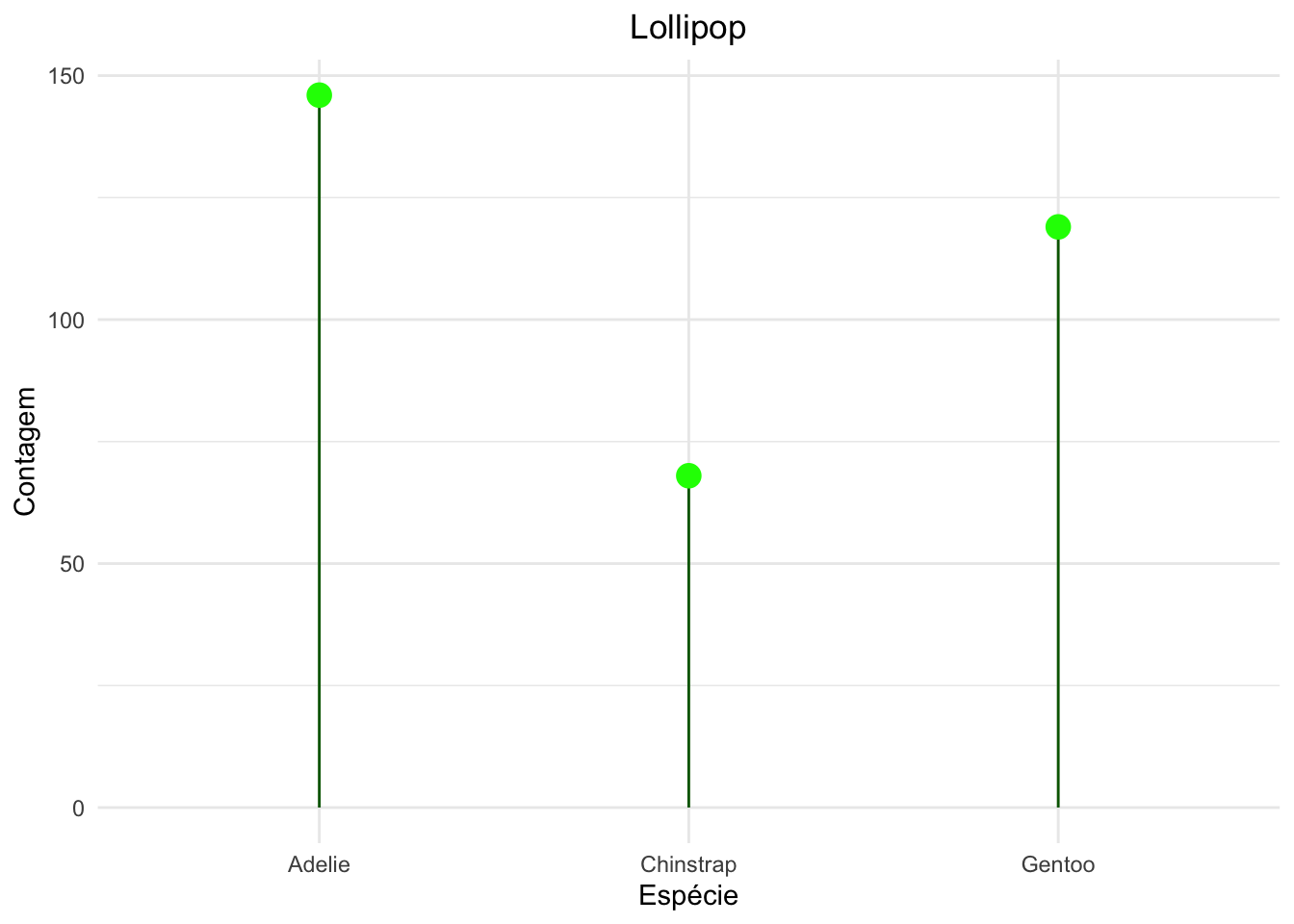
# Lollipopdf_count <- dados1 %>%count(species)(g2 <-ggplot(df_count, aes(x = species, y = n)) +geom_segment(aes(x = species, xend = species, y =0, yend = n), color ="darkgreen") +geom_point(size =4, color ="green") +labs(title ="Lollipop", x ="Espécie", y ="Contagem") +theme_minimal() +theme(plot.title =element_text(hjust =0.5)))
4.7 Contagem de classes de uma variável categórica
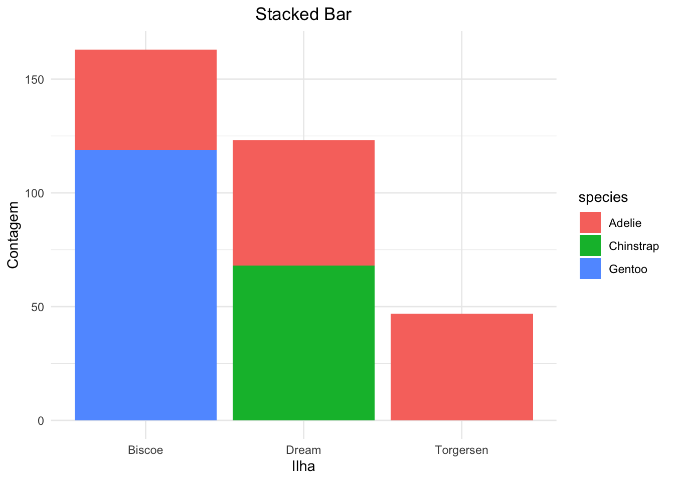
# Stacked bar(g1 <-ggplot(dados1, aes(x = island, fill = species)) +geom_bar(position ="stack") +theme_minimal() +labs(title ="Stacked Bar", x ="Ilha", y ="Contagem") +theme(plot.title =element_text(hjust =0.5)))
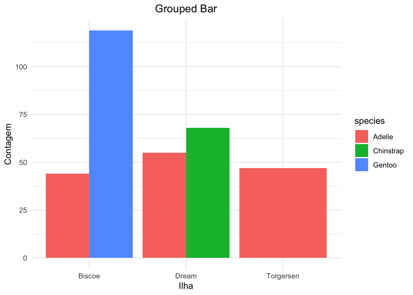
# Grouped bar(g2 <-ggplot(dados1, aes(x = island, fill = species)) +geom_bar(position ="dodge") +theme_minimal() +labs(title ="Grouped Bar", x ="Ilha", y ="Contagem") +theme(plot.title =element_text(hjust =0.5)))
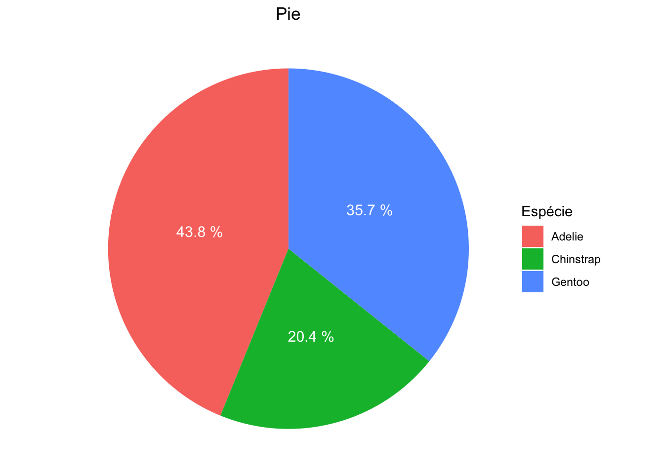
# Pie pie_data <- dados1 %>%count(species) %>%mutate(frac = n/sum(n), label =paste(round(100* frac, 1), "%"))(g3 <-ggplot(pie_data, aes(x="", y = frac, fill = species)) +geom_bar(stat ="identity") +coord_polar("y") +geom_text(aes(label = label),position =position_stack(vjust =0.5), color ="white", size =4) +theme_void() +labs(title ="Pie", fill ="Espécie") +theme(plot.title =element_text(hjust =0.5)))
4.8 Adição de estatísticas
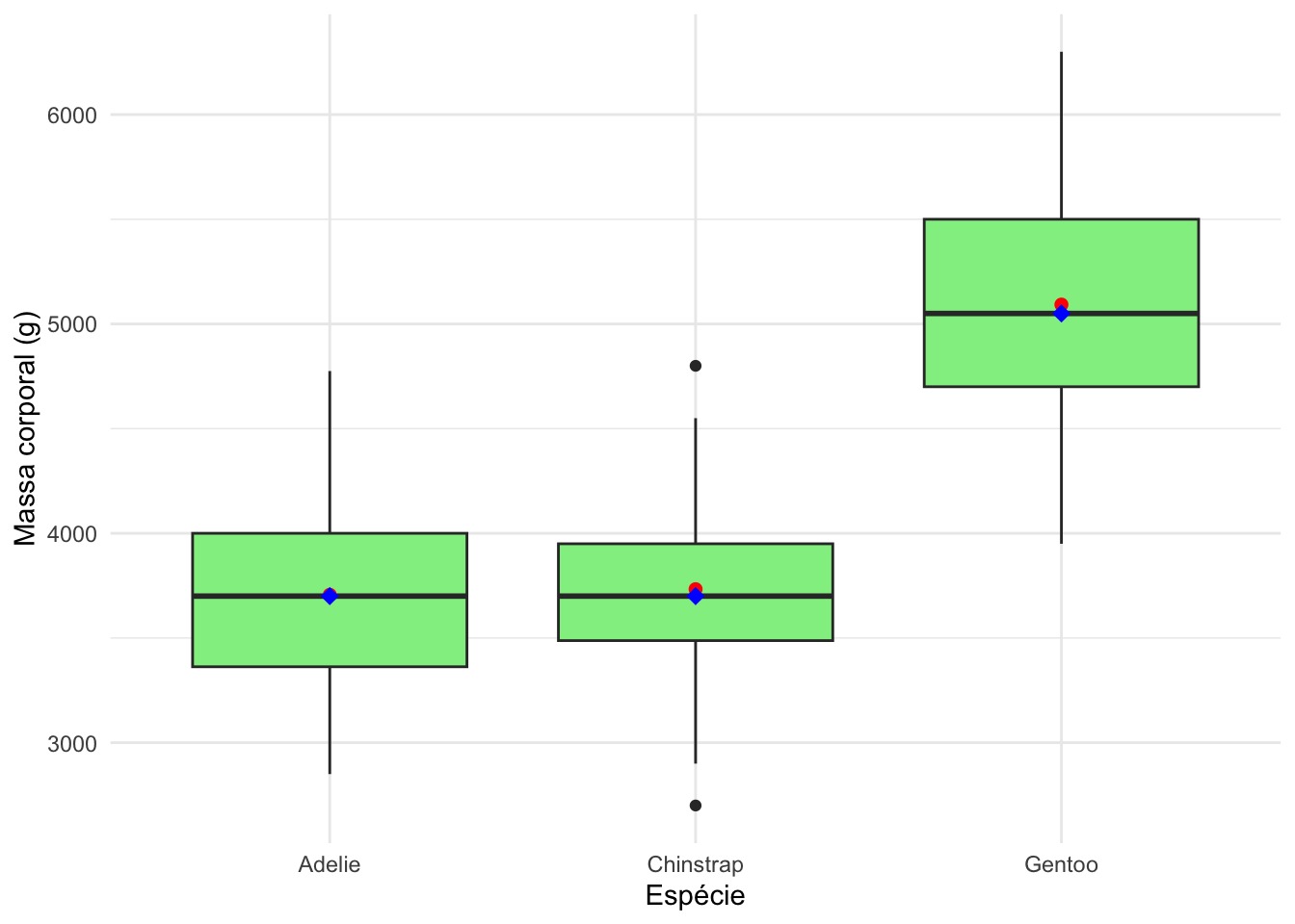
# Boxplot com média e medianaggplot(dados1, aes(x = species, y = body_mass_g)) +geom_boxplot(fill ="lightgreen") +stat_summary(fun = mean, geom ="point", shape =20, size =3, color ="red") +stat_summary(fun = median, geom ="point", shape =18, size =3, color ="blue") +labs(x ="Espécie", y ="Massa corporal (g)") +theme_minimal()
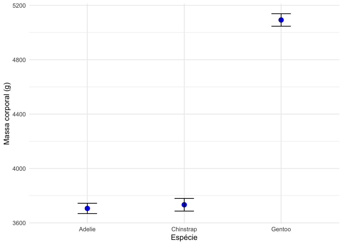
# Média ± erro padrão ggplot(dados1, aes(x = species, y = body_mass_g)) +stat_summary(fun = mean, geom ="point", size =3, color ="blue") +stat_summary(fun.data = mean_se, geom ="errorbar", width =0.2, color ="black") +labs(x ="Espécie", y ="Massa corporal (g)") +theme_minimal()
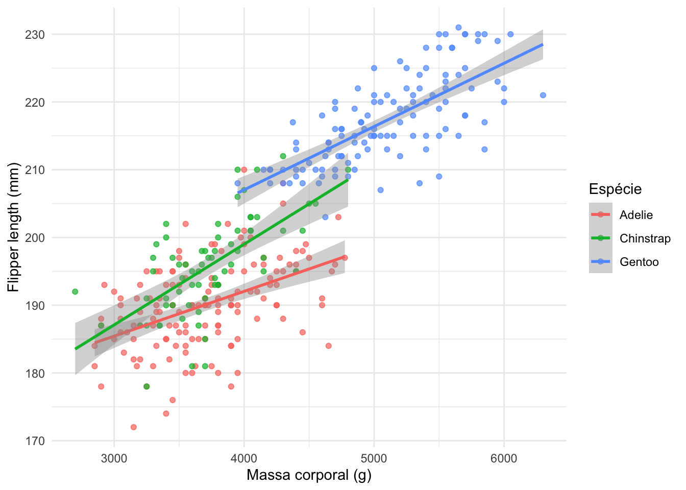
# Regressão linear: flipper_length_mm ~ body_mass_gggplot(dados1, aes(x = body_mass_g, y = flipper_length_mm, color = species)) +geom_point(alpha =0.7) +geom_smooth(method ="lm", se =TRUE) +labs(x ="Massa corporal (g)", y ="Flipper length (mm)", color ="Espécie") +theme_minimal()
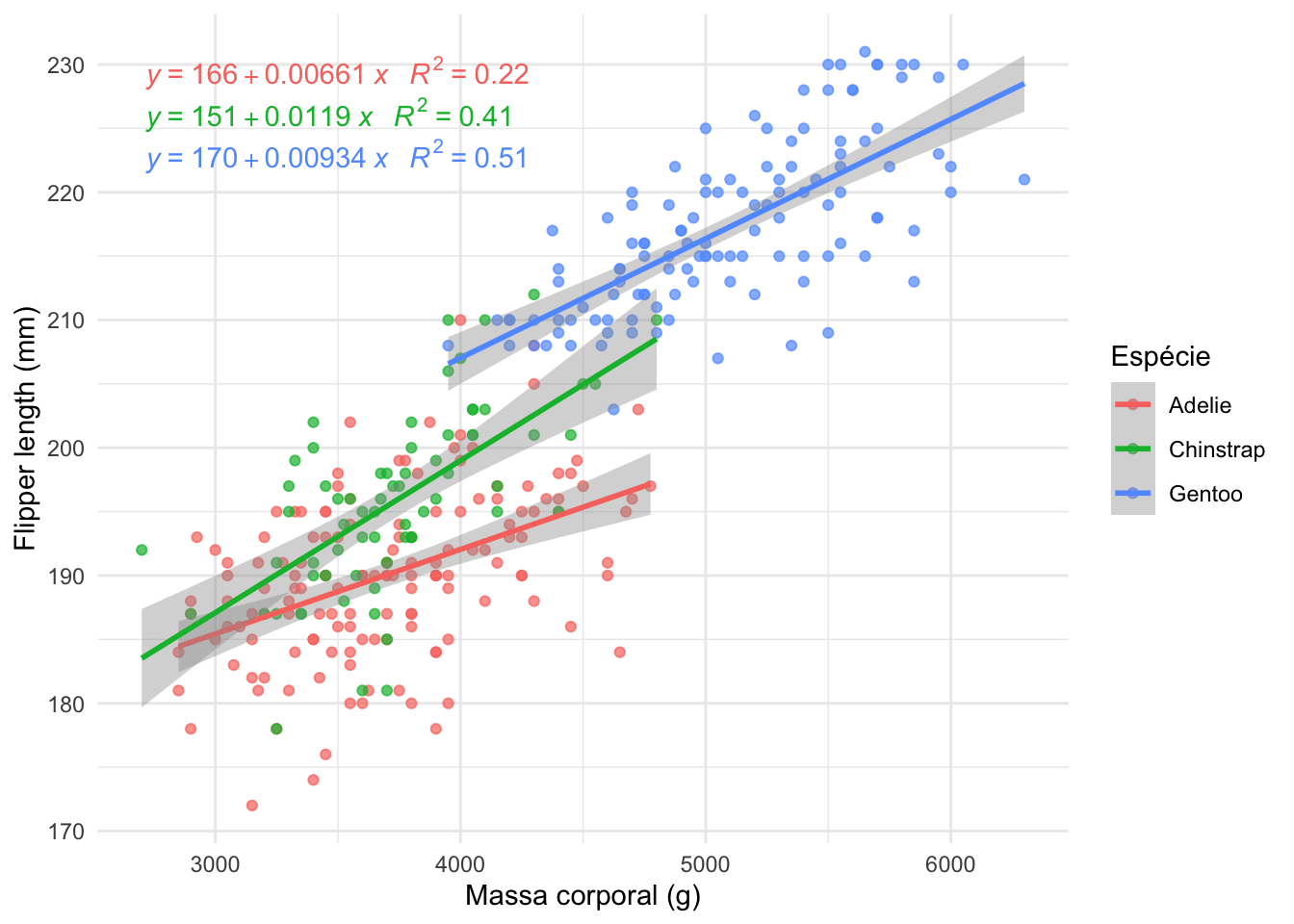
library(ggpmisc)ggplot(dados1, aes(x = body_mass_g, y = flipper_length_mm, color = species)) +geom_point(alpha =0.7) +geom_smooth(method ="lm", se =TRUE) +stat_poly_eq(aes(label =paste(..eq.label.., ..rr.label.., sep ="~~~")),formula = y ~ x, parse =TRUE, label.x.npc ="left", label.y.npc =0.95) +labs(x ="Massa corporal (g)", y ="Flipper length (mm)", color ="Espécie") +theme_minimal()
Pacotes específicos para gráficos com estatísticas: